[tutorials & resource material arranged by topic Class Table Class Table

Hypothesis Tests


Read Hypothesis Tests (How to Complete a Hypothesis Test)

pdf file
Table of Contents for CALCULATORing
Table of Contents for MIDDLE GROUND, Statistics
TI83-84 STATISTICS and DISTRIBUTION Menus

Testsignificance test for:test statistic
(observed"new") - (expected"old")
(test) =
(standard error)

Z-Test1 mean, normal, large sample sizeztest = ( - µ)/(/(n))

T-Test1 mean, small sample, sigma unknownttest = ( - µ)/(s/(n))

2 Sample Z-Test2 means

2 Sample T-Test2 INDEPENDENT means

2 Sample T-Test2 DEPENDENT means

ANOVA Test3 or more means using variances

1 Proportion Z-Test  1 proportion

2 Proportion Z-Test2 proportions

2 Testdiscrete (catagories)
Independence of Proportion
Is the preference independent of the group?

CREATE an EXPECTED
(row,column) distribution.

2 Testdiscrete (catagories)
Homogeneity of Proportions
Are preferences of subgroups the same?

CREATE an EXPECTED
(row,column) distribution.

Linear Regression
T-Test   
1 correlation coefficient, between x and y

2 GOF TestGoodness of Fit, match
"test" distribution to another distribution  

2 GOF TestNormality, match
"test" distribution to a normal distribution  

CREATE an EXPECTED distribution.

2 Test1 Variance 2test = [(n-1)s2]/2

Two Sample F Test2 variances

Sign Test1 median
or 1 pair, as in (After) - (Before) >0
not very sensitive a test

Wilcoxon
Mann-Whitney
Rank Sum Test
2 distributions
for symmetry, center, distribution of ranks
with averaged ranks awarded to tied data points

Wilcoxon
Signed-RankTest
median of 2 distributions
before-after
small sample size, not nec. normal


Z-Test Uses the Normal or Gaussian Probability Density Function or Distribution

This tests to see if evidence exists that the real mean is not the stated mean.
Needed:
n > 30
or, distribution is normal and standard deviation is known.
The null hypothesis is always:
H0: µ = (stated mean of the population)
The alternate hypothesis is always one of these:
H1: µ < (stated mean of the population)
H1: µ = (stated mean of the population)
H1: µ > (stated mean of the population)
Test statistic:
ztest = ( - µ)/(/(n))
Levels of confidence:
To Run a Calculator Confidence Interval to Test: (for 2-tail test)
[STAT], then [TESTS], then 7:Z-Interval...
To Run a Calculator Hypothesis to Test:
[STAT], then [TESTS], then 1:Z-Test...
One page Summary, sample problem, and a spreadsheet.


T-Test
This tests to see if evidence exists that the real mean is not the stated mean.
Needed:
approximately normal distribution,
unknown population standard deviation.
n< 30.
the larger the sample size, the closed the distribution approaches normal.
degrees of freedom, symbolized d.f., equals n-1.
The null hypothesis is always:
H0: µ = (stated mean of the population)
The alternate hypothesis is always one of these:
H1: µ < (stated mean of the population)
H1: µ = (stated mean of the population)
H1: µ > (stated mean of the population)
Test statistic:
ttest = ( - µ)/(s/(n))
Levels of confidence:
found in table organized by 1-tail or 2-tail and d.f.
or by calculator
To Run a Calculator Confidence Interval to Test: (for 2-tail test)
[STAT], then [TESTS], then 7:TInterval...
To Run a Calculator Hypothesis to Test:
[STAT], then [TESTS], then 2:T-Test...
One page Summary, sample problem, and a spreadsheet.


1 Proportion Z-Test
Used to test claims concerning percents, probabilities, proportions.
as in "70% of the population," "42% of the products"
Needed:
p, the population proportion, the stated proportion
= x/n, the sample proportion
np>5, nq>5, where q= 1- p
The null hypothesis is always:
H0: p = (stated proportion), may be symbolized as p0
The alternate hypothesis is always one of these:
H1: p (stated proportion)
H1: p < (stated proportion)
H1: p > (stated proportion)
Test statistic:
Levels of confidence:   as above z-test
or by calculator
To Run a Calculator Confidence Interval to Test: (for 2-tail test)
[STAT], then [TESTS], then A:1-PropZInterval...
To Run a Calculator Hypothesis to Test:
[STAT], then [TESTS], then 5:1-PropZTest...
One page Summary, sample problem, and a spreadsheet.


Linear Regression T-Test
This tests to see if evidence exists that there is a correlation
between the independent variable, x, and the dependent
variable, y. The populaltion correlation coefficient, rho,
symbol , is the strength of the linear relationship between x and y.
The relationship ranges between
a strong negative relationship (as x increases, y decreases)
to a weak relationship, to no relationship (0),
to a weak positive relatioship (as x increases, y increases),
to a strong positive relationship.
-1 < r < 1
 
Needed:
r, the sample correlation coefficient is
d.f. = n-2
The null hypothesis is always:
H0: = 0
The alternate hypothesis is always one of these:
H1: < 0     H1: 0     H1: > 0
Test statistic:
Levels of confidence:
found in table organized by 1-tail or 2-tail and d.f.
To Run a Calculator Confidence Interval to Test: (for 2-tail test)
[STAT], then [TESTS], then G:LinRegTInt...
To Run a Calculator Hypothesis to Test:
[STAT], then [TESTS], then F:LinRegTTest...
One page Summary, sample problem, and a spreadsheet.


2 Sample Z-Test
This tests to see if evidence exits that there is a difference between 2 means.
Needed:
two populations with known standard deviations.
independence between samples.
normal or approximately normal distributions if sample sizes are less than 30.
The null hypothesis is always:
H0: µ1 = µ2 or H0: µ1 - µ2 = 0
The alternate hypothesis is always one of these:
H1: µ1 µ2 or H1: µ1 - µ2 0
H1: µ1 > µ2 or H1: µ1 - µ2 > 0
H1: µ1 < µ2 or H1: µ1 - µ2 < 0
Test statistic: [Because the null hypothesis is µ12=0, the numerator is simplified!]
Levels of confidence:
or by calculator
To Run a Calculator Confidence Interval to Test: (for 2-tail test)
[STAT], then [TESTS], then 9:2SampZInterval...
To Run a Calculator Hypothesis to Test:
[STAT], then [TESTS], then 3:2SampZ-Test...
One page Summary, sample problem, and a spreadsheet.


2 Sample T-Test, Independent Samples
This tests to see if evidence exits that there is a difference between 2 means.
Needed:
two populations, means and standard deviation need not be known.
sample standard deviations must be known.
independence between samples and are not matched or paired,
normal or approximately normal distributions if sample sizes are less than 30.
The null hypothesis is always:
H0: µ1 = µ2 or H0: µ1 - µ2 = 0
The alternate hypothesis is always one of these:
H1: µ1 µ2 or H1: µ1 - µ2 0
H1: µ1 > µ2 or H1: µ1 - µ2 > 0
H1: µ1 < µ2 or H1: µ1 - µ2 < 0
Test statistic: [Because the null hypothesis is µ12=0, the numerator is simplified!]

Levels of confidence:
    d.f. smaller of n1-1 and n2-1
    or by weighted degrees of freedom
    as shown at right and in spreadsheet.
To Run a Calculator Confidence Interval to Test: (for 2-tail test)
[STAT], then [TESTS], then 0:2-SampTInt...
To Run a Calculator Hypothesis to Test:
[STAT], then [TESTS], then 4:2SampTTest...
One page Summary, sample problem, and a spreadsheet.


2 Sample T-Test, Dependent Samples, Paired, Before/After

      This tests hypothises about the mean of the
difference of paired samples. It's great for before
and after samples. Clearly the samples are not independent, but paired one-to-one to create
differences which become the sample statistics.
      This mean one is testing to see if there is a statistically significant difference before and after
some treatment or event.
Needed:
D = x1 - x2 for every pair of n samples
they are n matched or paired samples, as in before and after samples
each population is normal or approximately normal
d.f. = n-1
The null hypothesis is always: H0: µD = 0 (, or some constant)
The alternate hypothesis is always one of these:
H1: µD < 0 (, or some constant)
H1: µD 0 (, or some constant)
H1: µD > 0 (, or some constant)
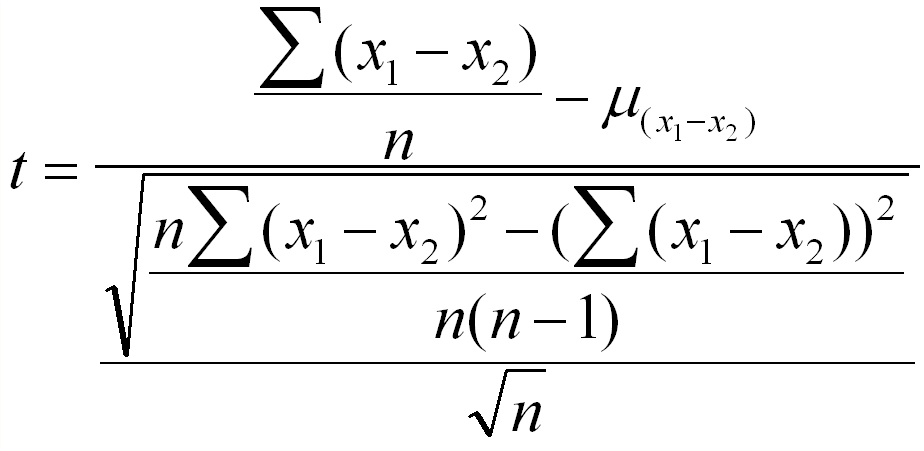
Test statistic: [Because the null hypothesis is µ12=0 or some constant,
the numerator may be simplified!]
Levels of confidence:
found in table organized by 1-tail or 2-tail and d.f.
To Run a Calculator Hypothesis to Test:
Create a list of the D distribution using D = x1 - x2 for every pair of n samples
then [STAT], then [TESTS], then 2:T-Test... on this D distribution
One page Summary, sample problem, (calculator version), and a spreadsheet.


2 Proportion Z-Test
    Used to test claims concerning 2 percents, probabilities,
proportions, as in "70% of males," vs "42% of females."
Needed:
samples are independent
n1p1 >5     n1q1 >5       n2p2 >5     n2q2 >5
The null hypothesis is always:
H0: p1 = p2
The alternate hypothesis is always one of these:
H1: p1 > p2       H1: p1 p2       H1: p1 < p2
Test statistic:
   
Levels of confidence:
To Run a Calculator Confidence Interval to Test: (for 2-tail test)
[STAT], then [TESTS], then B:2-PropInterval...
To Run a Calculator Hypothesis to Test:
[STAT], then [TESTS], then 6:2PropZ-Test...
One page Summary, sample problem, and a spreadsheet.


2 Test for A Single Variance
      This tests to see if evidence exists that
the real variance is not the stated variance.
      It's a test for consistency, hoping for little,
but enough, variation.
Needed:
normal population
random sample of n independent observations
population standard deviation and sample standard deviation
degrees of freedom, d.f. = n-1
The null hypothesis is always:
H0: 2 = (stated population variance)
The alternate hypothesis is always one of these:
H1: 2 < (stated population variance)
H1: 2 (stated population variance)
H1: 2 > (stated population variance)
Test statistic:
2test = [(n-1)s2]/2
Levels of confidence:
found in table organized by 1-tail or 2-tail and d.f.
CAN'T Run a Calculator Hypothesis to Test w/o a program
CAN Use [CATALOG] and 2cdf( in a program
8:2cdf(lower bound,upperbound,degrees of freedom)
One page Summary, sample problem, and a spreadsheet.


2 Test for Independence of Proportions
      This tests to see if evidence exists that the preferences of the
groups is independent of the group making the choice.
 
Needed:
Radom sample of full population is sorted by groups and their
preferences, usually sorted into rows and columns and
called a contingency table.
each cell of table must be 5 or greater or groups/preferences must be pooled
degrees of freedom, d.f. = ((rows)-1)((columns)-1)
The null hypothesis is always:
H0: The preference is independent of the group.
The alternate hypothesis is always:
H1: The preference is dependent on the group.
Test statistic: EXPECTED value table must be generated first using
the ratio:(row sum)(column sum)((grand sum) for each cell in table.
Levels of confidence:
found in table organized by 1-tail or 2-tail and d.f.
To Run a Calculator Hypothesis Test:
[MATRIX] then edit OBSERVED and EXPECTED matrices,
then [STAT], then [TESTS], then C:-Test...
One page Summary, sample problem, and a spreadsheet.


2 Test for Homogeneity of Proportions
      This tests to see if evidence exists that the one or more of the subgroup
in a population has a diferent distribution of proportions than the other subgroups.
 
Needed:
each subgroup is randomly sampled,
preferences are sorted into rows and columns called a contingency table
each cell of table must be 5 or greater or groups/preferences must be pooled
degrees of freedom, d.f. = ((rows)-1)((columns)-1)
The null hypothesis is always:
H0: psubgroup1 = psubgroup2 = psubgroup3 = ... = plast subgroup
The alternate hypothesis is always:
H1: One or more of the ps is different.
Test statistic: EXPECTED value table must be generated first using the ratio:
(row sum)(column sum)((grand sum) for each cell in the contingency table.
Levels of confidence:
found in table organized by 1-tail or 2-tail and d.f.
To Run a Calculator Hypothesis Test:
[MATRIX] then edit OBSERVED and EXPECTED matrices,
then [STAT], then [TESTS], then C:-Test...
One page Summary , sample problem, and a spreadsheet.


2 Goodness of Fit Test
      This tests to see if the observed result compares
favorably to the theoretical (or prior) results.
It also tests if a distribution is normal.
      The test looks at, all at once, how the
frequency distributions of observed catagories
compares to their expected frequencies.
      It answers the question: "Does the observed
result fit the pattern that was predicted?"
Recall that a completely random pattern would
have about equal frequencies in each catagory.
Needed:
random sample of size n where n/(number of catagories) > 5
O = the observed frequency in each catagory
E = the expected frequency in each catagory, WHICH IS...
      based on a random distribution:     E = n/(number of catagories)
      based on a prior distribution:     E = (prior catagory percent)(n)
degrees of freedom, d.f. = (number of catagories) - 1
The null hypothesis is:
H0: The distribution is the same as the published distribution.
      (It's a reasonable fit.)
H0: The distribution is normally distributed.
The alternate hypothesis is:
H1: The distribution is not the same as the published distribution.
      (It's not a really good fit.)
H1: The distribution is not normally distributed.
Test statistic:
Levels of confidence:
found in table organized by 1-tail or 2-tail and d.f.
To Run a Calculator Hypothesis Test:
Enter the OBSERVED frequencies in one list and EXPECTED in a matching list.
[STAT], then [TESTS], then D:2-Test...
One page Summary, sample problem, and a spreadsheet.


2 Test for Normality
      The Chi Square Goodness of Fit Test is here used to see if a distribution is normal.
      Three steps are required.
1st: Compute the mean and standard deviation
of the OBSERVED data (green).
2nd:Create an EXPECTED distribution using
the normal cumulative distribution function
and the OBSERVED mean and st.dev.(blue).
3rd: Run a GOF test using the OBSERVED and
EXPECTED distribution frequencies (purple).
The p in the test below is .619. The null hypothesis is confirmed. The OBSERVED bistribution is normal.

One page Summary and a spreadsheet.


Two Sample F-Test
This tests to see if evidence exists that two variances differ.
Needed:
2 normal distributions
independent samples
sample standard deviations
number in each sample
d.f.n. (numerator) = nnumerator-1
d.f.d. (denominator) = ndenominator-1
The null hypothesis is always:
H0: larger2 = smaller2
The alternate hypothesis is always one of these:
H1: larger2 < smaller2
H1: larger2 smaller2
H1: larger2 > smaller2
Test statistic:
Levels of confidence:
found in tables organized by d.f.n and d.f.d.
To Run a Calculator Confidence Interval to Test: (for 2-tail test)
[STAT], then [TESTS], then 7:TInterval...
To Run a Calculator Hypothesis to Test:
[STAT], then [TESTS], then 2:T-Test...
One page Summary, sample problem, and a spreadsheet.


ANOVA -- Analysis of Variance, One-Way, Single Factor
This tests to see if evidence exists that means of 3 or more groups differ when the variances are equal.
Needed:
population must be normal or near normal
independent samples
variances equal
N = n1 + n2 + n3 + ... + nk, k = the number of groups
d.f.numerator = k - 1
d.f.denominator = N - k
The grand mean, GM, is the mean of all data.
The null hypothesis is always:
H0: µ1 = µ2 = µ3 = ... = µk
The alternate hypothesis is always:
H1: One or more of the means is not equal to the others
Test statistic:
The F test statistic,
the sum of the squares between groups is SSB, (SSB)/(k-1) = MSB = sbetween2
the sum of the squares within groups is SSW, (SSW)/(N-k) = MSW = swithin2
  
Levels of confidence:
found in table organized by alpha, d.f.numerator, d.f.denominator
To Run a Calculator Hypothesis to Test:
[STAT], then [EDIT] to enter lists, then [STAT], [TESTS], then H:ANOVA(L1, L2, L3, ... ,Llast)
Page one of Summary, page 2 of Summary , sample problem, and a spreadsheet.


Sign Test
      This is really a binomial (+ or - response) test to see if evidence exists that a median is the
hypothesized median (single sample) or to see if a difference exists in paired data. If n is less than 26,
a formula is not used, just a count and compare procedure.  If n is greater than 25, a z-test is used.
In either case, the smaller of the number of data points above the median and number of data points
below the mean is used to compute the test statistic.
Needed:
a sample of 100 to do the job a sample of 30 does w/a more efficient test
may be nonparametric (not defined mean, standard deviation, etc.)
random sample
use the raw data to find the "sign" of [(data)-(stated median)]
Compute each [(data)-(stated median)] or [(After)-(Before)] first to determine n = x+ + x- !!!
The null hypothesis always:
      H0: median = (stated median)       or      H0: (After) - (Before) = 0
The alternate hypothesis is always one of these:
      H1: median < (stated median) H1: (After) - (Before) < 0
      H1: median = (stated median) H1: (After) - (Before) = 0
      H1: median > (stated median) H1: (After) - (Before) > 0
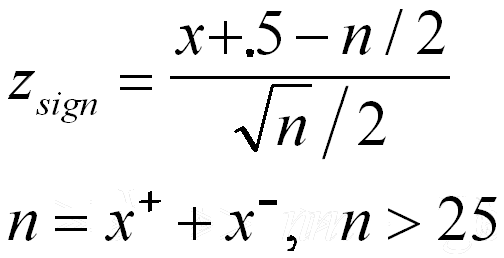
Test statistic:
      When n < 26, n = sum of x+ and x-       or      When n > 25, n = sum of x+ and x-
      smaller of:
    x+, the # of data points greater than median (or 0)
and
    x-, the # of data points less than the median (or 0)
      binomial distribution used where p=.5,
n = the sum of x+ and x-.
The z table is used with x in formula as
the smaller x+ and x-.
One page Summary , sample problem, and a spreadsheet.


Wilcoxon Rank Sum Test
This tests to see if evidence exists that 2 distributions are the same by virtue of
their symmetry, center, and the distribution of ranks (with averaged ranks awarded
to tied data points). Do two populations have the same distribution, are their centers
and spreads the same?
Needed:
2 not necessarily normal distributions
each sample size is 10 or greater
independent random samples
The null hypothesis is always:
H0: The distributions are the same.
    (The means and rank sums are "the same.")
Some alternate hypothesis are:
H1: The distributions are not the same.
  Are the means and rank sums close but not "the same?" ( )
H1: The first distributions is to the left of the other.
  Is the first's rank sums much smaller, data points more to the left, than the second's? ( < )
H1: The first distributions is to the right of the same.
  Is the first's rank sums much larger, data points more to the right, than the second's? ( > )
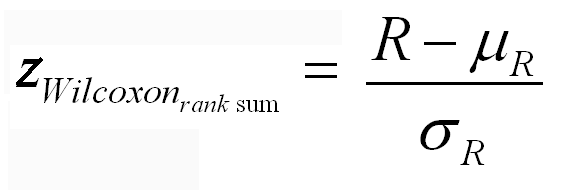
Test statistic: The sample size determines the labels in the formulas.
The label n1 is given to the smaller sample size -- fewer numbers to add.
The data is then POOLED, with averaged ranks awarded to tied data points.
Individual r1 and r2 are computed by adding the ranks of the data points from the samples.
R is r1, the sum of the ranks of the sample with the smaller sample size.
One page Summary , sample problem, and a spreadsheet.


Wilcoxon Signed-Rank Test
This tests to see if evidence exists that the medians of two distributions
are the same, or before-after differences exist.
Needed:
n samples paired as x1 - x2 = difference 0.
the ranks of the pooled absolute values of the differences, tie ranks averaged.
"signed-rank" products = (original sign)(pooled rank)
the absolute value of the sum of the products of the
    (original sign)(pooled rank) of the negative differences.
the absolute value of the sum of the products of the
    (original sign)(pooled rank) of the positive differences.
the SMALLER of the absolute values of the sums of the + or - signed-rank products
2 not necessarily normal distributions
independent random samples
The null hypothesis is always:
H0: median1 = median2, or H0: before - after = 0
Some alternate hypothesis are:
H1: median1 median2, or H1: before - after 0
H1: median1 > median2, or H1: before - after > 0
H1: median1 < median2, or H1: before - after < 0
Test statistic:
if n < 30, use table for critical value and the SMALLER for the test statistic
if n > 30, use z distribution for critical value and formula
    with µ = n(n+1)/4 for test statistic OR
if n > 30, use z distribution for critical value and
    the absolute value of the sum of all (sign)(rank) in formula
    with µ = .5 for test statistic
     
One page Summary , sample problem, and a spreadsheet.


Spearman rank correlation coefficient

Kruskal-Wallis test


[MC,i. Home] [Good Stuff] Classes [Words]
© 8/2012 A. Azzolino
www.mathnstuff.com/math/spoken/here/2class/90/htest2.htm